Start with a concrete routing problem, build a mixer that meets its constraints, and separate what the algebra guarantees from what experiments must establish.
Six connected learning units · Complete technical material · Illustrated reading edition
Start with the question you have
A connected route through the ideas
Read the six units in order for the full argument, or use the entry points below. Each unit begins with an explanation of the question it answers, then develops the original examples, derivations, and qualifications.
The reference sections can be opened when needed. Diagrams remain beside the explanations that use them; select “Enlarge diagram” for a closer view. Earlier section links still work.
Keep the main distinctions in view
d counts residual streams; D counts features; s sets the internal block size. A is skew-symmetric, Q is orthogonal, and B is the final routing matrix. The batch-size B used in the original tensor-shape notation is a separate quantity from the mixer B.
1. Start with the routing problem
Think of a residual stream as a feature vector that survives from one
layer to the next. With one stream, the familiar update keeps that
vector and adds a learned correction. With several streams, there is a
new decision to make before discussing the learned
correction: which old streams contribute to each new
stream?
Fix one token in one batch item. Its state can be written as a matrix
\(X\in\mathbb{R}^{d\times D}\): one row
per stream and one column per feature. A residual mixer \(B\in\mathbb{R}^{d\times d}\) acts on the
left, so \(BX\) mixes streams without
changing the feature dimension. The same routing weights apply to every
feature coordinate in this local calculation. The layer may compute
different weights from different activations; this notation describes
one realized mixer.
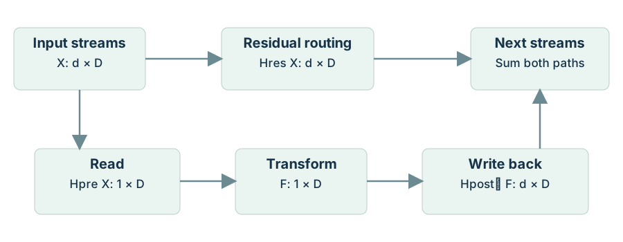
There are two paths through a Hyper-Connection layer. The residual
path mixes the existing streams directly. The learned branch first
reads a combination of streams, applies the ordinary
layer transformation, and then writes that result back
to the streams. The two paths are added. Keeping these roles separate
prevents a common mistake: the doubly stochastic constraint studied here
belongs to the residual mixer, not automatically to every coefficient in
the read–transform–write branch.
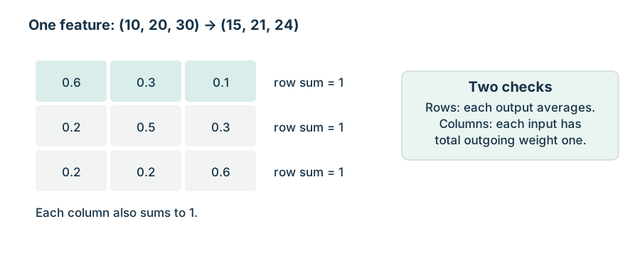
For a first numerical picture, let a single feature have values \(x=(10,20,30)^\top\). The three-stream
matrix in the worked example below produces \(Bx=(15,21,24)^\top\). The first output is
\(0.6(10)+0.3(20)+0.1(30)=15\).
Repeating that calculation for the other rows gives the other outputs.
The sum remains \(60\), but the three
values are redistributed. We will explain the two constraints
responsible for this behavior in the next unit.
This example is a generic valid routing matrix, not
a claim that the particular matrix belongs to every go-mHC family. First
understand what a mixer does; only then ask which mixers a
parameterization can produce.
The constraint concerns the residual-routing box. The read–transform–write branch is separate and is added afterward.
The problem: how
should residual streams mix?
Residual connections make deep networks trainable by providing a path
through which information and gradients can move without passing
exclusively through a sequence of nonlinear transformations. In its
simplest form, a residual update is
\[
x_{l+1}=x_l+\mathcal{F}(x_l,W_l),
\]
where \(x_l\) is the state at layer
\(l\), \(\mathcal{F}\) is a learned layer
transformation, and \(W_l\) denotes its
parameters.
Hyper-Connections generalize this construction by maintaining several
parallel residual streams rather than one. Let \(d\) be the number of streams. A layer can
then learn how to route information among those streams instead of using
a fixed identity connection. This makes \(d\) a possible capacity dimension,
analogous in spirit to depth or width: increasing \(d\) gives the model more pathways through
which information may travel.
The central difficulty is that repeated unrestricted stream mixing
can destabilize a network. If each layer applies an arbitrary mixing
matrix, repeated products can amplify or attenuate components of the
state and its gradients. Manifold-Constrained Hyper-Connections (mHC)
address this by constraining the residual mixing matrix to be doubly
stochastic [Xie et al., 2026].
The paper studied here proposes go-mHC, a direct
parameterization of a family of exactly doubly stochastic matrices. Its
purpose is to occupy a middle ground:
more expressive than highly structured Kronecker-factorized
mixers;
less expensive than parameterizing arbitrary doubly stochastic
matrices through all permutation matrices;
exact by construction, rather than only approximately satisfying the
constraint after iterative normalization.
The construction rests on generalized orthostochastic matrices
[Gutkin, 2013; Nechita et al., 2023].
From residual
connections to Hyper-Connections
A Hyper-Connection layer operates on a multi-stream state
The matrix is neither the identity nor a deterministic permutation.
It performs a soft redistribution of information while conserving total
routing mass.
A permutation matrix instead gives hard routing. For example,
This example exposes a limitation of restrictive factorized
constructions: a parameterization built only from \(2\times 2\) real-spectrum factors may fail
to express such a three-cycle. The cycle has nonreal cube roots of unity
among its eigenvalues, whereas \(2\times
2\) doubly stochastic factors have only real nontrivial
eigenvalues.
2. Understand the constraint and its limits
Two distinct conservation statements are hidden in the phrase “doubly
stochastic.” A row sum of one says that each output is a weighted
average of input streams. A column sum of one says that, across all
outputs, each input contributes total weight one. Nonnegativity makes
“weighted average” the right description rather than an arbitrary signed
cancellation.
The distinction is easiest to see with a counterexample. The
matrix
has row sums one, yet sends \((2,10)^\top\) to \((2,2)^\top\). Both outputs copy the first
input; the second input disappears. Its column sums are \(2\) and \(0\), so it is not doubly stochastic.
Checking only the rows misses the problem.
For a doubly stochastic mixer and any real feature vector \(x\),
The first identity preserves the sum across streams for that feature.
The second preserves a feature that already has the same value in every
stream. These are algebraic identities, so they do not require the
feature values themselves to be nonnegative.
Non-amplification
is not preservation of every direction
It preserves \((1,1)^\top\), but
sends \((1,-1)^\top\) to zero. It is
exactly doubly stochastic and still destroys the difference between the
streams. Therefore the constraint does not promise that
all information survives, or that gradients cannot vanish in any
direction. It controls amplification by the realized residual-routing
operator; it does not give a positive lower bound on every singular
value.
The norm statements below can also be read directly. Each output
coordinate is an average, so \(\|Bx\|_\infty\leq\|x\|_\infty\). Column
sums and the triangle inequality give \(\|Bx\|_1\leq\|x\|_1\). These bounds survive
products of doubly stochastic mixers. They are useful guarantees, but
they do not include the derivative of an activation-dependent mixer, the
learned branch, normalization, or the entire network Jacobian.
What “exact” means in an
implementation
Exact-by-construction describes the real-arithmetic formula. A
floating-point implementation still has rounding and linear-solve
errors. Test row and column residuals numerically rather than expecting
literal bitwise equality to one. The advantage is that there is no
separate finite-iteration normalization error to trade against a
stopping budget; ordinary numerical error still needs to be
measured.
Read rows to calculate outputs; read columns to check total input contribution. Both checks are required.
Why constrain the residual
mixer?
With unconstrained Hyper-Connections, \(\mathcal{H}_l^{\mathrm{res}}\) can in
principle be any learned matrix. This permits flexible routing but
removes an explicit identity-like guarantee.
Repeated application yields a cumulative routing operator
If the factors are unrestricted, this product can have directions
that grow or shrink rapidly. Such amplification or contraction can
contribute to exploding or vanishing gradients.
mHC constrains residual mixing toward the Birkhoff polytope using
finite Sinkhorn–Knopp normalization. Sinkhorn normalization alternates
row and column rescaling of a nonnegative matrix. The supplied
formulation uses twenty iterations.
This gives two practical concerns:
the iterative projection may require specialized implementation for
efficiency;
a finite number of iterations need not produce an exactly doubly
stochastic matrix.
A small violation at each layer may compound across depth. Exact
parameterizations seek to eliminate this particular source of
accumulated constraint error.
Stability and cumulative
mixing
For any nonnegative doubly stochastic matrix \(B\),
Nonnegativity is also preserved under matrix multiplication.
Therefore exact doubly stochastic mixing guarantees that the
cumulative routing operator remains doubly stochastic at arbitrary
depth. This explains why AGM does not distinguish exact methods such as
go-mHC, mHC-lite, and KromHC: all satisfy the same relevant row- and
column-sum property.
It does not prove that the methods have equal
optimization behavior, equal representational capacity, or equal
real-world training performance. For those comparisons, the paper turns
to expressivity and convergence.
3. Build the mixer from orthogonal blocks
We now have a specification: produce a nonnegative matrix whose rows
and columns sum to one. go-mHC meets that specification indirectly. It
first builds an orthogonal matrix, whose rows and columns have known
squared lengths, and then converts those squared lengths into
nonnegative routing weights.
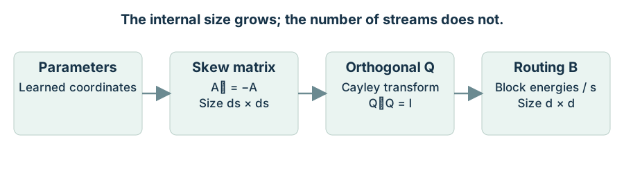
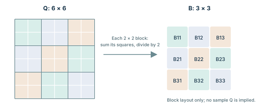
The sizes matter. There are \(d\)
actual residual streams. The orthogonal construction uses \(ds\) internal coordinates, grouped into
\(d\) blocks of \(s\) coordinates. Those extra coordinates
parameterize the mixer; they are not \(ds\) residual streams carried through the
network. After taking one normalized squared norm per block, the output
is again a \(d\times d\) matrix.
Why divide a block energy
by its size?
For \(s=1\), every row of an
orthogonal matrix has squared length one. For larger \(s\), a block row contains \(s\) ordinary orthogonal rows, each
contributing one unit of squared length. The total squared energy in the
whole block row is therefore \(s\).
Dividing its block energies by \(s\)
makes the corresponding routing row sum to one. The column argument is
the same. The proof below formalizes precisely this accounting
argument.
Notice what is discarded by the final map. The orthogonal matrix
contains signs and relationships between internal coordinates. The
routing matrix retains only block energies. Many different orthogonal
matrices can therefore produce the same mixer. Orthogonality of the
internal matrix does not imply that the final mixer
preserves vector length.
For \(x=(2,10)^\top\), the mixed
feature values are \((4.88,7.12)^\top\). Their sum is still
\(12\). The negative entry of \(Q\) causes no negative routing weight
because the final map squares it. This is a complete small instance of
the construction—not a numerical projection onto the constraint set.
The Cayley chart has a
boundary
A real skew-symmetric \(A\) cannot
make \(I+A\) singular. If \((I+A)v=0\), multiplying by \(v^\top\) gives \(\|v\|_2^2+v^\top Av=0\). Skew-symmetry
makes the second term zero, so \(v=0\).
Nevertheless, a finite Cayley parameterization does not cover every
orthogonal matrix: its output cannot have eigenvalue \(-1\), because \(I+Q=2(I+A)^{-1}\) is invertible. Thus the
full family obtained by allowing all orthogonal
matrices and the finite Cayley chart used to parameterize them must not
be casually identified. Nor does connectedness of a parameter space
prove that gradient descent reaches any desired target. The
construction, the representable family, and the behavior of an optimizer
are three separate questions.
Each map establishes a different property. The last map returns to d actual streams, regardless of the internal block size s.
Orthostochastic matrices
A matrix \(B\in\mathsf{B}_d\) is
orthostochastic if there exists an orthogonal matrix
\(Q\in\mathbb{R}^{d\times d}\) such
that
\[
B_{ij}=Q_{ij}^{\,2}.
\tag{6}
\]
Because squares are nonnegative, \(B_{ij}\geq 0\). Orthogonality gives
For \(d>2\), the orthostochastic
matrices form a proper, nonconvex subset of \(\mathsf{B}_d\). They include permutation
matrices but do not generally fill the polytope interior.
This produces the central idea behind go-mHC:
ordinary orthostochastic matrices correspond to \(s=1\);
a block generalization indexed by \(s\) expands the representable family;
as \(s\to\infty\), that family
approaches the full Birkhoff polytope.
Generalized
orthostochastic matrices
A block row contains two unit-length orthogonal rows. Its total squared energy is two; division by two gives one routing row.
Let
\[
Q\in\mathcal{Q}(ds)
\]
be an orthogonal \(ds\times ds\)
matrix. Partition it into a \(d\times
d\) block matrix, with each block
This differs fundamentally from iterative normalization:
Sinkhorn begins with a matrix and repeatedly corrects it toward the
constraint;
go-mHC parameterizes a matrix family that satisfies the constraint
by construction.
4. Choose a representation and a cost
Once several methods all meet the same row and column constraints,
“which method is stable?” is too coarse a question. Compare three things
separately: the set of routing matrices available, the cost of producing
one of them, and the behavior of the optimization that chooses among
them.
mHC-lite starts from deterministic routings and blends them. A
Kronecker construction builds a large routing pattern from smaller
factors. go-mHC builds an internal orthogonal matrix and measures its
block energies. These are different restrictions on the
representation of a mixer, even when their outputs
satisfy the same constraints.
The factorial cost described below belongs to the parameterization
that assigns a component to every permutation. The Birkhoff–von Neumann
theorem itself does not require an implementation to enumerate all
permutations in order to describe a particular target. It is the chosen
learnable full enumeration that incurs that cost.
Increasing \(s\) enlarges the
internal construction from \(ds\)
coordinates to a larger system. At \(d=4\), the skew generator has \(6\), \(28\), or \(66\) independent entries for \(s=1,2,3\), respectively. This is a useful
concrete scale before reading the complete parameter-count formulas.
Those formulas also include the network that predicts the generator, so
the generator count alone is not the layer’s total parameter count.
Treat block size as a hypothesis to test, not a default quality
score. A larger internal matrix may reduce representation error but
costs more to construct and differentiate. Better geometric coverage
does not guarantee that a fixed optimizer, initialization, and training
budget will exploit it.
The practical comparison should hold the task, stream count,
precision, optimization budget, and hardware conditions fixed. Report
constraint residuals and target-reconstruction error separately from
elapsed time. A loss curve against optimization steps answers a
different question from a loss curve against wall-clock time.
Existing exact alternatives
mHC-lite:
complete coverage at factorial cost
mHC-lite uses the Birkhoff–von Neumann representation. Because every
doubly stochastic matrix is a convex combination of permutation
matrices, mHC-lite can in principle cover the full Birkhoff
polytope.
Its cost is the number of permutations:
\[
d!.
\]
The source reports a parameter cost on the order of
\[
\mathcal{O}(dC\cdot d!),
\]
where \(C\) is a model-dependent
feature or projection cost. This is exact and expressive, but factorial
growth makes it unsuitable for large \(d\).
KromHC: efficient factorization with restricted routing
KromHC constructs a large mixer using Kronecker products of smaller
doubly stochastic matrices. For matrices
the Kronecker product \(A\otimes B\)
is an \(mp\times nq\) block matrix
whose \((i,j)\)-th block is \(A_{ij}B\).
If the factors are doubly stochastic, their Kronecker product is also
doubly stochastic. This gives exact constraint satisfaction with a
highly structured parameterization.
The cost is lower, but the structure strongly limits which large
mixing matrices can be represented. The paper’s key criticism is
spectral: products of small factors need not acquire the rich complex
spectral behavior available to general matrices in \(\mathsf{B}_d\).
go-mHC is intended to improve this trade-off: it is more expressive
than a small-factor Kronecker construction while avoiding factorial
enumeration.
The role of the block size \(s\)
The parameter \(s\) controls the
block size in the orthogonal matrix \(Q\).
\(s=1\): ordinary
orthostochastic matrices;
larger \(s\): more
orthogonal degrees of freedom before block energies are aggregated;
\(s\to\infty\):
asymptotic approach to the full Birkhoff polytope.
The paper uses \(s=2\) as its
principal default and compares it with \(s=1\) and \(s=3\).
This produces a direct efficiency–expressivity dial.
Smaller \(s\)
Smaller \(s\) gives fewer parameters
and lower computation. At \(s=1\), a
\(d\times d\) skew-symmetric generator
has only
\[
\frac{d(d-1)}{2}
\]
independent parameters.
But \(s=1\) is restricted to the
orthostochastic subset. For \(d>2\),
this subset does not fill the interior of \(\mathsf{B}_d\).
Larger \(s\)
Larger \(s\) gives a broader family
of generalized orthostochastic matrices. The source reports that
increasing \(s\) yields denser spectral
coverage, with \(s=2\) covering a
larger region than \(s=1\).
The trade-off is that the orthogonal matrix has size \(ds\times ds\), so linear algebra on it
becomes more expensive.
Complexity trade-offs
Let:
\(d\): number of residual
streams;
\(C\): a model-dependent channel or
projection-cost factor;
\(s\): generalized-orthostochastic
block size;
\(S\): number of Sinkhorn
iterations;
\(i_k\): Kronecker factor
size.
Parameter counts
The source gives the following total parameter-count forms:
The principal comparison is therefore not “fast versus slow” in
isolation.
mHC-lite gives broad exact coverage but grows factorially.
KromHC is highly efficient but structurally restricted.
mHC may have lower nominal polynomial order but requires iterative
projection.
go-mHC pays cubic dependence on \(d\) to obtain an exact, direct, and more
expressive constrained family.
For the source’s nominal illustrative setting,
\[
S=20,
\qquad
i_k=2,
\qquad
s\in\{1,2\}.
\]
These are configuration choices, not universal constants. Measured
runtime also depends on memory traffic, batch size, tensor layout,
linear-solve implementation, and hardware parallelism.
Combining go-mHC and
KromHC
The paper presents go-mHC and KromHC as complementary rather than
mutually exclusive.
A possible combined strategy is:
use Kronecker factorization to represent a large stream-mixing
structure efficiently;
use generalized orthostochastic factors rather than only small
conventional doubly stochastic factors;
increase factor size \(i_k\)
without immediately paying a factorial \(i_k!\) cost.
The reported intuition is that factorized structure controls
large-scale computation, while go-mHC enlarges the local family of exact
doubly stochastic transformations available inside each factor.
This does not eliminate the fundamental restrictions of
factorization. It changes the trade-off by making each factor more
expressive.
5. Interpret spectra and experimental evidence
An eigenvalue describes what a fixed linear mixer does to one mode
under repeated application. An eigenvalue of one preserves the mode. A
real eigenvalue with magnitude below one damps it; a negative one also
alternates its sign. A nonreal conjugate pair describes a
two-dimensional real subspace with rotational behavior. These statements
concern repeated application of a fixed operator, not a complete
nonlinear language model.
The spectral obstruction in the discussion below can be made
dimensionally explicit. To compare with a \(2\times2\) Kronecker factorization, embed a
three-cycle in four streams:
This matrix cycles three streams and leaves the fourth fixed. Its
eigenvalues are \(1,1,e^{2\pi i/3},e^{4\pi
i/3}\). By contrast, a mixer of the form \(A\otimes B\), with two \(2\times2\) doubly stochastic factors, has
only real eigenvalues. That particular factorization cannot represent
\(C_4\). This is an obstruction for the
stated mixer family, not a theorem that any larger architecture using
small factors can never perform cyclic computation.
The synthetic experiment asks a different question: given inputs and
outputs generated by a known matrix, can optimization learn the
transformation? A useful interpretation separates three sources of loss:
noise in the targets, a target outside the representable family, and
failure of the optimizer to find a good point inside that family.
Reaching a noise floor on a sampled task is evidence for that task; it
does not prove every matrix is representable or every training problem
is easy.
Read the evidence in three layers. The nonnegativity and row/column
identities are algebra. Spectral plots and reconstruction curves are
measurements under a specified sampling and optimization procedure. A
claim about better language models requires language-model results and
an appropriate compute comparison. Keeping these layers separate makes
the paper’s useful construction easier to assess without making it carry
a stronger claim than the evidence supports.
Spectral reach
as an expressivity surrogate
The full volume of the Birkhoff polytope is difficult to use directly
as an expressivity measure. The paper therefore evaluates
spectral reach: the set of eigenvalues obtainable from
matrices produced by a given parameterization.
For a method \(\mathsf{M}\) with map
\(\mathcal{P}_{\mathsf{M}}\), the
spectral reach concerns eigenvalues \(\lambda\in\mathbb{C}\) such that
The relevant ambient region is the Karpelevič
region: the set of complex eigenvalues attainable by stochastic
matrices of a given dimension.
Because doubly stochastic matrices are stochastic, their eigenvalues
must lie in this region. A method with broader spectral reach can
realize a broader range of decay, persistence, oscillation, and cyclic
behavior under repeated application.
This is a useful surrogate, but it has an important limitation:
Broad spectral coverage does not prove that every doubly stochastic
matrix is representable.
Different matrices can share eigenvalues. Thus spectral reach is
evidence about dynamic diversity, not a complete volume or coverage
proof.
Reported qualitative
findings
For \(d=3\), the source reports
that:
\(s=1\) covers a substantial
spectral region, including the real interval \([-1,1]\), but leaves an error gap \(\epsilon(s=1)\);
\(s=2\) covers a larger region with
smaller reported gap,
\[
\epsilon(s=2)<\epsilon(s=1).
\]
For \(d=4\), the reported comparison
is:
finite-iteration mHC can contain points outside the desired doubly
stochastic region;
mHC-lite nearly fills the boundary-compatible region;
KromHC occupies only a highly restricted slice;
go-mHC with \(s=1\) covers a
sizable but incomplete region;
go-mHC with \(s=2\) fills a larger
and denser region.
These are empirical spectral observations, not proofs of exact
finite-\(s\) polytope coverage.
Why
Kronecker products have a spectral limitation
Let \(A\) and \(B\) have eigenvalues \(\lambda_A\) and \(\lambda_B\), respectively. The eigenvalues
of the Kronecker product \(A\otimes B\)
are pairwise products:
\[
\lambda(A\otimes B)
=
\left\{
\lambda_i(A)\lambda_j(B)
\right\}_{i,j}.
\]
For a \(2\times 2\) doubly
stochastic matrix, the spectrum has the form
\[
\operatorname{spec}(A\otimes B)
=
\{
1,\lambda_A,\lambda_B,\lambda_A\lambda_B
\}.
\tag{14}
\]
All four values remain real and lie in \([-1,1]\).
This has a direct consequence: repeated Kronecker composition from
\(2\times 2\) doubly stochastic factors
cannot generate genuinely complex eigenvalues. It therefore cannot
represent dynamics that require nonreal eigenvalues, including directed
cyclic behavior such as a three-cycle.
The latter two are nonreal. Hence a real-spectrum \(2\times 2\)-factor construction cannot
represent that cycle exactly.
The limitation is not merely aesthetic. In a recurrently applied
mixing operator:
real eigenvalues correspond to non-oscillatory expansion,
contraction, or sign reversal;
complex eigenvalues permit rotational or cyclic components.
The paper interprets this as a distinction between diffusion-like
mixing and directed, advective, or periodic routing behavior.
Synthetic
reconstruction experiment
The controlled experiment constructs:
ground-truth doubly stochastic matrices \(T_i\);
dense residual-stream activations \(X_j\);
noisy targets
\[
Y_{i,j}=T_iX_j+\xi,
\tag{15}
\]
where \(\xi\) is noise.
A learned parameterization is evaluated by how well it reconstructs
the transformation that generated \(Y_{i,j}\).
This is a useful design because the target transformation is known.
Reconstruction error can therefore isolate whether the parameterization
can reach and optimize toward the intended stream-mixing map.
The abstract reports that go-mHC reaches the minimum theoretical loss
on synthetic stream-mixing tasks and converges up to \(10\times\) faster than the compared
parameterizations. This should be read as an experimental result under
the source paper’s task construction and optimization configuration, not
as a universal convergence theorem for all architectures and
datasets.
The paper also reports validation in a GPT-style language model with
approximately \(30\) million
parameters. A GPT-style model is an autoregressive Transformer that
predicts each token from preceding context using causally masked
self-attention.
What is theoretically established, empirically observed, and still
uncertain?
Theoretical or algebraic
facts
The following statements follow from the construction or stated
mathematical results:
If \(Q\) is orthogonal, then \(\Phi_{d,s}(Q)\) is doubly stochastic.
At \(s=1\), generalized
orthostochastic matrices reduce to ordinary orthostochastic
matrices.
Products of doubly stochastic matrices remain doubly
stochastic.
The generalized orthostochastic family is contained in \(\mathsf{B}_d\).
The cited result of Nechita et al. states asymptotic approach to
\(\mathsf{B}_d\) as \(s\to\infty\).
Kronecker-product eigenvalues are products of factor
eigenvalues.
Experimental
observations reported by the source
The following are reported results rather than consequences of the
definitions:
\(s=2\) has a smaller reported
spectral gap than \(s=1\) in the
illustrated setting;
go-mHC reaches the reported theoretical minimum on the synthetic
task;
go-mHC converges up to \(10\times\)
faster in the reported synthetic comparisons;
the method was tested in a \(30\)M-parameter GPT-style language
model.
Four important open or
incomplete points
Finite-\(s\) coverage
bounds.
The source states that the generalized family approaches the full
Birkhoff polytope as \(s\to\infty\),
but the supplied material does not provide a practical bound on the
approximation error \(\epsilon(s)\) for
finite \(d\) and finite \(s\).
Convergence guarantees versus
representability.
The paper refers to proofs concerning coverage, path connectedness, and
gradient stability in an appendix. Those proofs are not included here.
In particular, a claim that every admissible target can be reached must
be interpreted carefully for fixed finite \(s\), because finite-\(s\) generalized orthostochastic families
can remain strict subsets of \(\mathsf{B}_d\).
Spectral reach is incomplete as an expressivity
metric.
Spectral coverage can reveal important restrictions, especially the
inability to represent cyclic modes, but it cannot establish full
matrix-space coverage. Nonidentical matrices can have identical
spectra.
Implementation-level and language-model evidence is
incomplete in the supplied material.
The source states that no custom CUDA kernels are required and reports a
\(30\)M GPT-style validation, but the
complete hyperparameters, measured language-model outcomes, hardware
conditions, and reproducibility details are not available in the
material presented here.
Conclusion
go-mHC reframes constrained residual-stream mixing as a composition
of geometric maps:
Its central advantage is exactness by construction. The block-energy
map \(\Phi_{d,s}\) converts an
orthogonal matrix into a valid doubly stochastic routing matrix without
iterative Sinkhorn normalization.
The parameter \(s\) is the essential
design variable. It interpolates between the restricted orthostochastic
regime at \(s=1\) and increasingly
expressive generalized orthostochastic families as \(s\) grows. This permits a controlled
compromise between computational cost and reachable stream-routing
behavior.
Relative to mHC-lite, go-mHC avoids factorial enumeration of
permutation matrices. Relative to KromHC, it can represent a broader
family of spectral and routing behaviors. Relative to finite-step
Sinkhorn-based mHC, it provides an exact direct map, though its cubic
dependence on stream count creates a separate computational cost.
The strongest conceptual lesson is that residual-stream capacity is
not determined only by the number of streams. It is also determined by
the geometry of the matrix family allowed to mix them.
6. Review the mathematics and test the construction
The main route has used four mathematical ideas: weighted averages,
orthogonal matrices, blockwise squared norms, and eigenmodes. The
original prerequisites are collected here for a slower review, followed
by the exercises and references. Open the part you need; there is no
need to restart the whole article because one symbol is unfamiliar.
A small numerical audit
The following NumPy example implements the map with a linear solve
rather than forming an explicit inverse. Rows of blocks are the output
streams; columns of blocks are the input streams.
import numpy as npdef residual_mixer(raw, streams, block_size): n = streams * block_size raw = np.asarray(raw, dtype=float)if raw.shape != (n, n):raiseValueError("raw must have shape (streams * block_size,) * 2") A = (raw - raw.T) /2 identity = np.eye(n) Q = np.linalg.solve((identity + A).T, (identity - A).T).T blocks = Q.reshape(streams, block_size, streams, block_size) B = np.sum(blocks * blocks, axis=(1, 3)) / block_sizereturn Q, BA = np.array([[0, 1/3], [-1/3, 0]])Q, B = residual_mixer(A, streams=2, block_size=1)assert np.allclose(Q.T @ Q, np.eye(2))assert np.all(B >=0)assert np.allclose(B.sum(axis=0), 1)assert np.allclose(B.sum(axis=1), 1)assert np.allclose(B, [[0.64, 0.36], [0.36, 0.64]])assert np.allclose(B @ [2, 10], [4.88, 7.12])
These checks test the construction, not training performance. A
training implementation must also test differentiation through the
solve, its chosen precision, and its initialization. In particular, at
\(A=0\), the squared-entry map has zero
first-order change: off-diagonal entries of \(Q\) begin at zero and are squared, while
the diagonal has no first-order skew perturbation. Identity
initialization is therefore not automatically a useful initialization
for learning the residual mixer.
Mathematical prerequisites
Mathematical prerequisites
Doubly stochastic matrices
A square matrix \(B\in\mathbb{R}^{d\times
d}\) is doubly stochastic if:
\(B_{ij}\geq 0\) for every \(i,j\);
every row sums to one;
every column sums to one.
Equivalently, if \(\mathbf{1}\in\mathbb{R}^d\) is the all-ones
vector, then
The set of all \(d\times d\) doubly
stochastic matrices is the Birkhoff polytope,
denoted
\[
\mathsf{B}_d.
\]
A doubly stochastic matrix may be interpreted as a conservative
routing rule. Each output stream receives a nonnegative weighted
combination of input streams, and each input stream distributes one unit
of total mass across the outputs.
This does not mean every individual feature is preserved. Rather, it
means the routing matrix cannot arbitrarily create or destroy total
stream mass in the \(\ell_1\)-style row
and column senses.
Permutation matrices and the Birkhoff–von Neumann theorem
A permutation matrix has exactly one entry equal to
\(1\) in every row and every column,
with all other entries equal to \(0\).
It represents deterministic routing: each input stream is sent to
exactly one output stream.
The Birkhoff–von Neumann theorem states:
Every doubly stochastic matrix is a convex combination of permutation
matrices.
where \(S_d\) is the set of all
\(d!\) permutations and \(P_\pi\) is the associated permutation
matrix.
This theorem gives an exact parameterization of \(\mathsf{B}_d\), but it creates a severe
scaling problem: there are \(d!\)
permutation matrices. At \(d=8\),
\[
8!=40{,}320.
\]
A representation that assigns a learned component to every
permutation therefore becomes impractical quickly.
Orthogonal and
skew-symmetric matrices
A matrix \(Q\in\mathbb{R}^{n\times
n}\) is orthogonal when
\[
Q^\top Q=I.
\]
Orthogonal matrices preserve Euclidean length:
\[
\lVert Qv\rVert_2=\lVert v\rVert_2.
\]
A matrix \(A\) is
skew-symmetric when
\[
A^\top=-A.
\]
Its diagonal entries must be zero, and only the entries above one
diagonal are independent. Thus an \(n\times
n\) skew-symmetric matrix has
\[
\frac{n(n-1)}{2}
\]
independent parameters.
The Cayley transform maps an appropriate skew-symmetric matrix into
an orthogonal matrix:
\[
Q=(I-A)(I+A)^{-1}.
\]
For skew-symmetric \(A\), \(I+A\) is invertible over the reals, and
\(Q\) is orthogonal. The transform
parameterizes the special orthogonal component reachable without
reflections, which is useful because that component is path
connected.
Exercises
Exercise 1: Verify
double stochasticity
Let \(Q\in\mathbb{R}^{ds\times ds}\)
be orthogonal and partitioned into \(s\times
s\) blocks \(Q_{ij}\). Prove
directly that
Write the permutation matrix for the routing cycle
\[
1\to 2\to 3\to 1.
\]
Find its eigenvalues. Explain why a construction whose spectrum is
restricted to real values cannot represent this cycle exactly.
Exercise 4: Compare growth
rates
Compute
\[
d^3
\quad\text{and}\quad
d!
\]
for \(d=4,6,8,10\). At what point
does the practical difference become obvious?
References
Dandachi, T., & Diggs-Galligan, S. (2026). go-mHC: Direct
Parameterization of Manifold-Constrained Hyper-Connections via
Generalized Orthostochastic Matrices. arXiv:2604.02309.
Gutkin, E. (2013). Work introducing generalized orthostochastic
matrices.
Nechita, I., et al. (2023). Results on generalized \(s\)-orthostochastic matrices and their
limiting coverage.
Xie, et al. (2026). Manifold-Constrained
Hyper-Connections.